Pulsed nuclear magnetic resonance on protons - Advanced lab course physical chemistry

Preliminary remarks

Nuclear Magnetic Resonance (NMR) methods are one of the most important analytical methods within chemistry and are indispensable for the analysis of molecular structures.

Even a very simple NMR experiment can be used to measure various resonance frequencies of protons, which allows to obtain information on the chemical composition of the sample. There are a number of more complex NMR experiments which can be used to unravel the spatial arrangement of molecular structures.

NMR has gained large popularity in the medical field as one of the most important imaging techniques. Nuclear magnetic resonance tomography allows to record 3D data sets of, i.e., the human body.

This lab course covers fundamental principles that are common to NMR methods. Simple NMR experiments are used to study the behavior of protons in a static magnetic field.

Theoretical foundations

Fundamentals – Zeeman splitting

Many atomic nuclei exhibit an intrinsic angular momentum $\vec{I}$ (spin) and thus exhibit a magnetic moment ^(†) $\vec{\mu}$ , according to

\vec{\mu} = \hbar\gamma\vec I

The gyromagnetic ratio $\gamma$ is specific for the used element and isotope. Hydrogen atoms $\ce{^1H}$ exhibit the largest gyromagnetic ratio with $\gamma_{\ce H} = 2\pi\cdot \pu{42.567e6s-1T-1}$ .

Nuclear magnetic resonance spectroscopy detects the magnetic properties of nuclei by detecting their interaction with an external magnetic field. In the simplest case the sample is placed in an external static magnetic field $\vec B_{0}$ . The interaction energy between a dipole moment $\vec \mu$ and an external magnetic field $\vec B_{0}$ can be expressed in a classical model as $E = - \vec{\mu}\cdot\vec B_{0}$ . It is common to align the direction of the external magnetic field with the $z$ axis, meaning that

\vec B_{0} = \begin{pmatrix} 0 \\ 0 \\ B_{0} \\ \end{pmatrix}

From a quantum mechanical treatment of the interaction between a nucleus and $\vec B_{0}$ it follows that only certain orientations of $\vec{\mu}$ relative to $\vec B_{0}$ are allowed. The interaction energy takes on discrete values,

E_{m} = - m\cdot\hbar\gamma B_{0}

where $m$ is the magnetic quantum number, which can take on values according to the nuclear quantum number $I$ :

m = + I, + (I - 1),\ldots , - (I - 1), - I

A proton $\ce{^{1}H}$ with a nuclear spin of $I = \frac{1}{2}$ allows two energy levels $E_{\frac{1}{2}}$ and $E_{-\frac{1}{2}}$ . The energy difference between the two states is labeled Zeeman splitting

\Delta E = E_{-\frac{1}{2}} - E_{\frac{1}{2}} = \hbar\gamma B_{0} = \hbar\omega_{\text L} = h\nu_{\text L}

and is proportional to the strength of the magnetic field. The angular frequency $\omega_{\text L}$ is called Larmor frequency ( $\omega_{\text L} = 2\pi\nu_{\text L}$ ).

A precise description of the interaction between the nucleus spin with external magnetic fields and with other nuclei is possible using quantum mechanics.

Here, we limit the discussion on a vector model that allows to describe simple relationships. Even simple spin-spin interactions (i.e., J-coupling) cannot be described using this vector model.

Thermodynamic equilibrium - Boltzmann statistics

Nuclei with a spin of $I=1/2$ (i.e. $\ce{^{1}H}$ , $\ce{^{13}C}$ ) can take on two states within a strong external magnetic field, corresponding to two opposite orientations along the $z$ axis. Of each individual spin, only the $z$ component of the spin $\mu_{z}$ and the length $\left| \vec{\mu} \right| = \sqrt{\mu_{x}^{2} + \mu_{y}^{2} + \mu_{z}^{2}}$ is determined.

For an ensemble of spins in thermodynamic equilibrium, a fraction of the spins with $m = +\frac{1}{2}$ contributes to the magnetization along the $z$ direction, while the rest ( $m = -\frac{1}{2}$ ) contributes in the opposite direction. According to Boltzmann statistics

\frac{N_{m = - \frac{1}{2}}}{N_{m = + \frac{1}{2}}} = e^{- \frac{\Delta E}{\text{kT}}}\qquad < 1

the effective total magnetization of the sample is $\vec{M} = \sum_{i}^{}{\vec{\mu}}_{i} > 0$ and points along the $z$ direction. In the magnet used in this lab course $\omega_{\text L} \approx 2\pi \cdot \pu{20MHz}$ follows from equation (6) at room temperature that $\frac{N_{-}}{N_{+}} = 0.99999672$ . The difference in occupation of the two states and, therefore, the total magnetization $|\vec{M}|$ is very small.

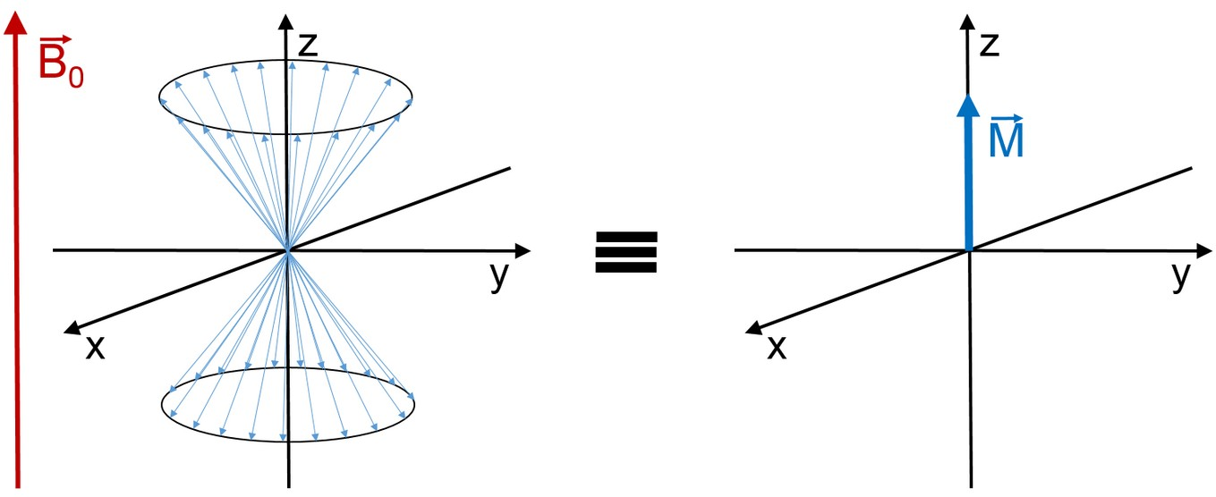
In thermodynamic equilibrium, the Zeeman splitting of the energy levels (small blue arrows, left) within an external magnetic field leads to an effective net magnetiziation (large blue arrow, right).

For a simple NMR experiment, the sum of all spins can be described using the vector model, which we will use in the following.

A simple NMR experiment

For conducting an NMR experiment, an additional magnetic field, perpendicular to $\vec B_{0}$ is introduced. Experimentally, a high-frequency coil is used to induce an oscillating magnetic field $\vec B_{1} (t)$ .

For an NMR experiment a sample is placed into the magnetic field

B_0

of a permanent magnet. Perpendicular to this static magnetic field, an oscillating magnetic field

B_1(t)

is applied with a matching transition frequency. After this excitation, the sample emits itself an oscillating magnetic field, which is detected by the same coil.

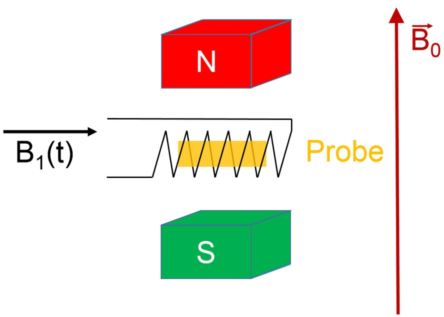
If a high-frequency pulse with a matching frequency $\omega_{\text L}$ is applied on the coil, transitions between the two energy levels of the nuclei can be induced (stimulated).

The action of a so-called $90\degree$ -pulse corresponds to a rotation of the total magnetization by $90\degree$ and can be expressed (with an additional step) using the vector model.

In thermodynamic equilibrium the net magnetization points in the same direction as the external magnetic field

B_0

. By irradiating a high-frequency pulse of certain energy, frequency and duration the magnetization can be rotated into the

xy

plane. The figure shows the magnetization in the rotating frame.

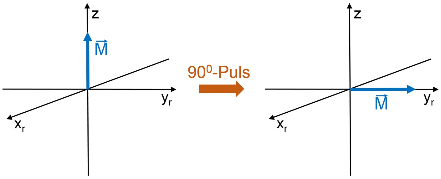
Indeed after the HF pulse the spins precess coherently with the Lamor frequency around the $z$ axis. Correspondingly, the magnetization $\vec{M}$ precesses after the HF pulse as well. If we, as an observer, rotate with the same frequency around the $z$ axis, the magnetization $\vec{M}$ seems to be time-independent. We performed a transformation from the fixed, inertial system $(x,y,z)$ to a rotating frame $(x_{r},y_{r},z)$ . A simple analogy can be made using a rotating carousel. In the lab frame the children pass the observer repeatedly. If the observer walks around the carousel matching its speed, the children remain stationary relative to the observer.

The macroscopic magnetization, which is precessing after the $90\degree$ pulse induces inside the HF coil a current that oscillates with frequency $\omega_{\text L}$ and results in a voltage $U(t) \propto \cos(\omega_{\text L} t)$ , which is called nuclear induction and is measured.

Mathematically, the transformation to a rotating frame can be performed by multiplying the measured voltage $U(t)$ with $\cos(\omega_{\text r} t)$ .

U_{r}(t) = U(t) \cdot \cos\left( \omega_{\text r}t \right) = U_{0}\cos\left( \omega_{\text L}t \right)\cos\left( \omega_{\text r}t \right)

= \frac{U_{0}}{2}\left\lbrack \cos\left( \left( \omega_{\text L}{- \omega}_{\text r} \right) t \right){+ \cos}\left( \left( \omega_{\text L} + \omega_{\text r} \right) t \right) \right\rbrack

The low-frequency component with frequency $\omega = \omega_{\text L} - \omega_{\text r}$ is processed further, while the high-frequency component $\omega = \omega_{\text L} + \omega_{\text r}$ is usually removed using a low-pass filter. In case that the rotating frame rotates exactly with the precession frequency, meaning $\omega_{\text L} = \omega_{\text r}$ , it follows that $U_{\text r}(t) \approx \frac{U_{0}}{2}$ is a time-independent signal.

If the rotating frame does not exactly match the precession frequency, i.e., if $\omega_{\text L}{\neq \omega}_{\text r}$ , we obtain a signal that oscillates with the frequency difference $U_{\text r}(t) \approx \frac{U_{0}}{2}\cos\left( \left( \omega_{\text L}{- \omega}_{\text r} \right)t \right)$ . In the simple carousel analogy this means that the observe moves slightly slower (or faster) besides the carousel. The children move relative to the observer, but only with the velocity difference.

Various effects lead to a decay of the nuclear magnetic induction over time. This decay of the magnetization in the $x,y$ plane is called free induction decay (FID) and results either from relaxation processes within the sample or from various local transition frequencies. $\omega_{\text L}$ .

The simplest reason for various local transition frequencies $\omega_{\text L}$ are inhomogeneities of the magnetic field, which are commonly present in magnets. Usually the inhomogeneity is reduced in NMR magnets by using additional coils which induce additional magnetic fields for correction. This is called shimming.

Inhomogeneities in the magnetic field mean that at different positions within the sample the magnetic field strength is different, which comes along that the Lamor frequencies $\omega_{\text L}$ are different as well. Since the rotating frame rotates with one exact frequency $\omega_{\text r}$ , one can observe a dephasing of the total magnetization after the $90\degree$ pulse.

Interactive visualization of the dephasing. The left-hand graph shows the FID signal, the right-hand graph shows at each timestep some spins as blue dots and the corresponding net magnetization as blue cross. The inhomogeneity of the magnetic field (

\Delta B_0

) can be adjusted using the slider. (The relaxation effects mentioned later in this document are modelled using

T_1 = \pu{1 s}, T_2 = \pu{100 ms}

B_0 = \pu{0.5T}

Influence of the pulse duration on the FID intensity

In thermodynamic equilibrium the total magnetization of the NMR sample is aligned with the z-direction. For achieving a maximum FID intensity, the HF pulse requires a certain power and duration. Typically, the power is fixed/given, which leaves the time duration of the HF pulse as a variable. The duration is adjusted such that the FID intensity is at its maximum. This corresponds to a rotation of 90°, as shown in figure 3. If the HF pulse duration would be doubled, the magnetization is rotated by an angle of 180° and no magnetization along the z axis (and no signal at the coil, see figure 2) would be detected.

Influence of the pulse duration (here expressed directly as pulse angle) on the magnetization measured by the coil. (The relaxation effects mentioned later in this document are modelled using

T_1 = \pu{1 s}, T_2 = \pu{100 ms}

Let us assume that the optimal pulse duration is $\pu{10\mu s}$ for rotating the magnetization by 90°. A pulse duration of $\pu{20\mu s}$ would lead to not observing a FID. A pulse duration of $\pu{30\mu s}$ , however, would rotate the magnetization by 270°, which would result in a maximum negative FID. A pulse duration of ${40\mu s}$ causes a 360° rotation and the total magnetization would point again along the +z direction (→ no FID). Pulse durations in-between the above values lead to shorter FID intensities.

Spectrum of a high-frequency pulse

To apply different frequencies to the sample at once, it is usually sufficient to emit one pulse with a single fixed frequency. The resulting pulse contains a spectrum of frequencies (see appendix, section 6).

For obtaining the frequency components of the time-domain signal, a Fourier transform is performed. This transform allows to convert a signal to its reciprocal domain. Here, a time signal [ $s$ ] is transformed to a frequency signal [ $s^{- 1}$ ]. This transform is without loss of information, meaning that the frequency-domain signal contains the same information as the time-domain signal and the transform and its inverse can be applied arbitrarily often without changing the signal.

If the pulse from figure is infinitely long, the Fourier transform yields a sharp line (delta function) at $\pu{20 MHz}$ . With decreasing pulse duration the line (spectrum) becomes broader.

A high-frequency pulse with a frequency of 20 MHz and a duration of

t = \pu{1\mu s}

contains 20 oscillations and corresponds to a spectrum with a FWHM of 1.2 MHz. (FWHM: full width half maximum)

A pulse with a length of $\Delta t = \pu{1 \mu s}$ results in a spectrum with a $\text{FWHM} = \pu{1.2 MHz}$ . A pulse with a duration increased by 10 fold, $\Delta t = \pu{10\mu s}$ , corresponds to a spectrum with $\text{FWHM} = \pu{120 kHz}$ . The shape of the spectrum with its multiple local maxima is determined by the Fourier transform of the rectangular function ( $\left| \frac{\sin(x)}{x} \right|$ ).

As a consequence for the NMR experiment, a pulse duration of $\pu{10\mu s}$ with a base frequency of $\pu{20 MHz}$ allows to effectively excite nuclei in the frequency range $\pu{19.940 MHz - 20.060 MHz}$ .

Chemical shift - NMR spectrum

If the external magnetic field $B_{0}$ is known, the resonance frequency of the protons can be calculated using equation 5. The equation only applies if the plain nucleus without electrons would be present. In atoms, the electrons cause additional magnetic fields, which increase or decrease (shield) the external magnetic field.

In the case of shielding, the outer (external) magnetic field $B_{0}$ induces with the electrons a secondary field $B_{\text{ind}}$ , which points in the opposite direction as the external field. The effective field at the nucleus $B_{\text{eff}}$ is therefore

B_{\text{eff}} = B_{0} - B_{\text{ind}} = \left| \ \vec B_{0} \right| - \left| \vec B_{\text{ind}} \right| = B_{0}\ (1 - \sigma)

The shielding constant $\sigma$ depends on the electron density at the nucleus. The larger the shielding constant, the larger is $\sigma$ . A smaller magnetic field causes a smaller Zeeman splitting (equation 5), which causes a shift towards lower frequencies by

\Delta\omega = \omega_{0}\sigma

To determine the shielding constant from a measured frequency, the frequency $\omega_{0}$ must be known precisely. In practice, NMR is not performed to determine absolute values for $\sigma$ , but to determine the shielding relative to a reference substance $\sigma_{\text{ref}}$ . The resonance frequency of the reference substance is

\omega_{\text{ref}} = \omega_{0}\ \left( 1 - \sigma_{\text{ref}} \right)\

The resonance frequency of the sample $\omega_{\text{sample}}$ relative to $\omega_{\text{ref}}$ is determined as chemical shift $\mathbf{\delta}$ (assuming $\sigma \ll 1$ ) with

\delta = \frac{\omega_{\text{sample}} - \omega_{\text{ref}}}{\omega_{\text{ref}}} = \frac{\sigma_{\text{ref}} - \sigma_{\text{sample}}}{1 - \sigma_{\text{ref}}} \approx \sigma_{\text{ref}} - \sigma_{\text{sample}}

A frequently used reference substance is tetramethylsilane (TMS). It consists of 12 equivalent protons, meaning that all protons exhibit the same electron density at the nucleus and therefore the same shielding constant. An additional benefit of TMS as reference substance is that the shielding of the protons in TMS is larger than in most common organic compounds, $\sigma_{\text{TMS}} > \sigma_{\text{sample}}$ . Since the chemical shift is typically rather small, it is expressed in $\text{ppm}$ (parts per million).

\delta = \frac{\sigma_{\text{ref}} - \sigma_{\text{sample}}}{1 - \sigma_{\text{ref}}} \approx \left( \sigma_{\text{ref}} - \sigma_{\text{sample}} \right)\ \cdot \ 10^{6}\text{\ ppm}

For protons $\ce{^{1}H}$ the value for $\delta$ is in the range from $\pu{0 ppm}$ to $\pu{15 ppm}$ .

To determine the chemical shift of a sample it is sufficient to emit a simple $90\degree$ pulse. After this pulse, the total magnetization in the xy plane dephases (figure 4). A voltage is induced in the coil (FID), which is then processed and analyzed.

Since the recorded voltage oscillates with a high-frequency component, first the signal is transformed in the rotating frame.

Example:

A mixture consisting to $99\%$ of benzene and to $1\%$ of TMS is measured. TMS is used as reference substance.

Now we assume that due to the specific magnetic field strength the protons of TMS exhibit a resonance frequency of $\omega_{\text{ref}} = 2\pi\cdot\pu{20.000000 MHz}$ . In the same magnet, the protons of benzene exhibit a resonance frequency of $\omega_{\text{benzene}} = 2\pi\cdot\pu{20.000146MHz}$ . Substituting the values in equation 11 yields a chemical shift of $\delta = \pu{7.3 ppm}$ .

For the excitation of the sample a pulse with a duration of $\pu{10 \mu s}$ with $\pu{20.000 MHz}$ is used, to excite nuclei in the range $\pu{19.940 MHz - 20.060 MHz}$ (see previous chapter).

The frequency range is broad enough to excite all protons within benzene and TMS. After the pulse, both species emit with $\pu{20.000000 MHz}$ and $\pu{20.000146 MHz}$ , respectively. Now we transform to the rotating frame, which rotates with $\pu{20.000000 MHz}$ . This corresponds to shifting the spectrum of the signal by the base frequency of $\pu{20.000000 MHz}$ , such that TMS exhibits a frequency of $\pu{0 Hz}$ and benzene a frequency of $\pu{146 Hz}$ in the rotating frame.

Upper graph: Time signal (FID) of a species (e.g. benzene at 146 Hz) in the rotating frame. The brown curve (real part) corresponds to the oscillating amplitude along the

y

axis, the red curve (imaginary part) along the

x

curve. The total amplitude is

\sqrt{I_\text{real}^2+I_\text{imag}^2}

.
Lower graph: Frequency signal of a species (e.g, benzene at 146 Hz) in the rotating frame. The width of the peak is essentially determined by the inhomogeneity of the used magnet (which is rather large for the magnet used in the lab course). (Relaxation effects are modelled using

T_1 = \pu{1 s}, T_2 = \pu{100 ms}

To identify these frequency components within the time-domain signal, a Fourier transform is performed (see Appendix). Thus, the time-domain signal $[\mathrm s]$ is transformed to a frequency-domain signal $[\mathrm s^{- 1}]$ .

Relaxation into thermodynamic equilibrium

In thermodynamic equilibrium the two Zeeman energy levels of a proton are occupied according to Boltzmann statistics (equation 6). The equilibrium occupation is perturbed after irradiating the sample with the high-frequency pulse and subsequently, the spin system relaxes in the thermodynamic equilibrium. Due to coupling between spin and environment the relaxation is called spin-lattice relaxation. The corresponding time constant is called $T_{1}$ . Sometimes the term longitudinal relaxation is used. In this case, longitudinal refers to the $z$ axis (see figure 3), the term transversal refers to the $xy$ plane.

There are various possibilities to measure the time constant $T_{1}$ . If the sample is in equilibrium, a $180\degree$ pulse can be used to rotate (invert) the total magnetization by $180\degree$ .

In thermodynamic equilibrium the total magnetization points in the direction of the external magnetic field

B_0

. A 180° pulse inverts the magnetization.

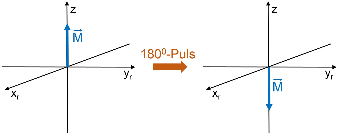
This means that there are now more spins in the energetically higher state than in the lower state. Thus, the spin system has to relax energy to the surroundings (lattice). The magnetization $\vec{M}$ relaxes again to the value according to the Boltzmann equilibrium.

The longitudinal magnetization relaxes exponentially into thermodynamic equilibrium. (The simulation assumes that

T_2 = \pu{100 ms}

. )

The time trace of the relaxation can not be captured using a single experiment. Instead, the relaxation time trace is obtained by perturbing the equilibrium magnetization (for example with a $180\degree$ pulse) and querying the magnetization after a time $t_{i}$ . This is repeated for many times $t_{i}$ .

The read-out of the magnetization is done with a second pulse, a $90\degree$ pulse, which rotates the longitudinal magnetization into the xy plane and, subsequently, induces a signal in the coil. The amplitude of the magnetization follows an exponential time law and is modeled here with

M(t) = M_{0} - 2M_{0} \cdot \ e^{- \ \frac{t}{T_{1}}}

Here, $M_{0}$ is the equilibrium magnetization, $M(t \rightarrow \infty) = M_{0}$ .

The relaxation time constant $T_{1}$ depends, among others, on the movement of the molecules in the sample! Transitions between nuclear spin states take place by stimulating with the required energy. This is what happens when a high-frequency pulse is applied using the high-frequency coil. However, state transitions can occur even without irradiating a HF pulse, but by the interaction between the protons. If a molecule moves into the neighborhood of a proton, the magnetic field at the proton fluctuates. This fluctuation is typically random and consists of multiple components at various frequencies, including a contribution at more or less $\pu{20 MHz}$ . A particularly effective spin-lattice relaxation, meaning a particularly small $T_{1}$ can be obtained if the movement of the molecules (rotation, translation) contains a particularly large amount of $\pu{20 MHz}$ . A good example is glycerol, which is rather viscous at room temperature and exhibits a large amount of $\pu{20 MHz}$ contributions. There is an optimal temperature at which the molecular movement of glycerol causes a minimum $T_{1}$ . At other temperatures, the values move either slower or faster, resulting in less of a $\pu{20 MHz}$ contribution and, consequently, an increase in $T_{1}$ .

Spin echo

The dephasing of the magnetization after a $90\degree$ pulse in the $xy$ plane (figure 4) is partially reversible! Particularly, the dephasing due to inhomogeneities of the magnetic field strength can be reversed. For this, after the $90\degree$ pulse an additional $180\degree$ pulse must be applied.

After the first pulse the magnetization dephases. At the time $t_\text{a}$ an echo pulse is applied. Since the rephasing takes an equal amount of time as the dephasing, at time $2t_\text{a}$ the echo signal can be detected.

Interactive visualization of the spin echo with FID signal (left) and the individual spins (right). First, a 90° pulse is emitted. If after some time

t_\text a

an additional 180° pulse is emitted, a spin echo

t_\text{a}

occurs at time

2t_\text a

. (Relaxation effects are modelled using

T_1 = \pu{1 s}, T_2 = \pu{100 ms}

Experimental setup

Hardware

In this lab course, a full-fledged NMR system is used, which even allows to perform 3d tomography recordings. The magnet is a permanent magnet. Besides its small magnetic field strength the temperature dependence of the field strength is a disadvantage.

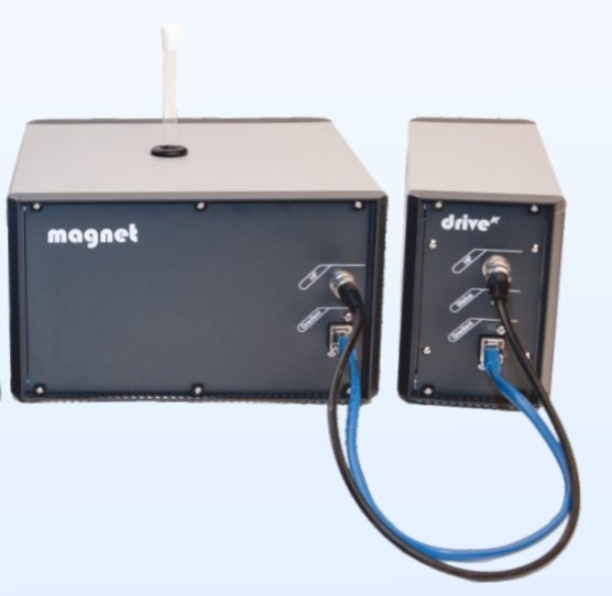
NMR spectrometer. Permanent magnet (links) and high-frequency electronics (rechts) are separated. The magnet has an opening for sample tubes with a diameter of at most 10 mm.

The spectrometer is connected to the computer via a USB cable and is controlled with a specialized software.

Software

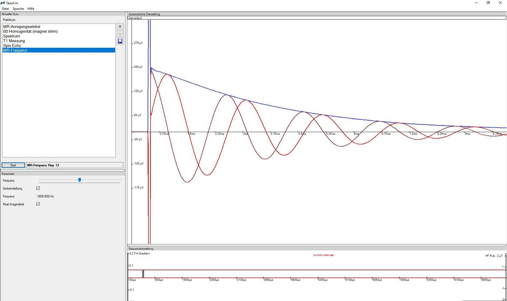
The software pd Teach’m controls the NMR spectrometer fully and allows to analyze the recorded data.

Experimental tasks and analysis

Go to virtual lab course

A variety of NMR experiments with different samples and NMR measurement protocols are performed.

Resonance frequency of glycerol

Determine the resonance frequency of glycerol and calculate the effective magnetic field strength $B_{\text{eff}}$ . Repeat this step at the end of the lab course.

NMR measurement protocol	MR frequency (MR-Frequenz)
Sample	Glycerol
Instructions	Change the frequency adjustment using the slider (either with the mouse or, even better, with the arrow keys). The time signal oscillates with the frequency difference between the selected MR frequency and the resonance frequency of the nuclei in the sample. You have found the resonance frequency if the deviation between the blue and brown curve is minimal.
Analysis	Make a note of the frequency and determine $B_{\text{eff}}$ and the Zeeman splitting as $\omega_{\text{eff}}$ and $E_{\text{eff}}$ . Estimate the uncertainty of the observed resonance frequency and discuss the changes of the frequency in the course of the measurement session.
Results	Time 1: $\nu_\text{eff} =$ $\omega_\text{eff} =$ $B_\text{eff} =$ $E_\text{eff} =$ Time 2: $\nu_\text{eff} =$ $\omega_\text{eff} =$ $B_\text{eff} =$ $E_\text{eff} =$

90°-pulse length

The sample is excited with a pulse and the signal strength is determined as function of the pulse length.

NMR measurement protocol	MR-Anregungswinkel
Sample	Glycerol
Instructions	Change the pulse length with the slider and determine using your eye (or a ruler) the signal intensity (blue curve). Take note of the pulse length at (a) maximum positive signal. Next, increase the pulse length in small steps until the signal becomes minimal (b). Next, determine the pulse length of a maximum negative signal (c).
Analysis	Take a note of all three pulse lengths. Do not forget to reset the pulse length to the value obtained for the 90° pulse!
Results	$t_1 =$ $t_2 =$ $t_3 =$

Shimming

Optimize the homogeneity of the magnet using the three shim coils in $X$ , $Y$ and $Z$ direction. The shim coils induce an additional magnetic field gradient, which allows to compensate inhomogeneities of the permanent magnet.

NMR measurement protocol	B0 Homogenität (magnet shim)
sample	Glycerol
Instructions	Change the gradient in $x$ , $y$ and $z$ direction such that the FID (blue curve) decays as slowly as possible.
Analysis	Make a note of the settings of the shim coils. What unit is used to express the inhomogeneity?
Ergebnisse	$\frac{\mathrm dB_0}{\mathrm dx} =$ $\frac{\mathrm dB_0}{\mathrm dy} =$ $\frac{\mathrm dB_0}{\mathrm dz} =$

Chemical shift

Determine the chemical shift of benzene and cyclohexane and use $B_{\text{ref}}$ and $\omega_{\text{ref}}$ (from 3.1) to calculate the corresponding resonance frequencies.

NMR measurement protocol	Spektrum
Samples	Benzol/TMS, Cyclohexan/TMS
Instructions	Record at least 20 spectra per sample and determine the average.
Analysis	Determine the chemical shift. Read the peak maximum by clicking it. Discuss the difference between benzene and cyclohexane. Why does cyclohexane show only a single maximum?
Results	$\delta_\text{benzene}=$ $\delta_\text{cyclohexane}=$

T₁-Relaxation

Determine the time it takes for the population of the energy states of the protons to relax to the distribution given by the Boltzmann equation.

NMR measurement protocol	T1 Messung
Samples	Glycerol, Ethylenglykol
Instructions	Change the parameters such that the relaxation curve is clearly visible. The time duration (repetition time) between the experiments should be at least $5 T_{1}$ . Record at least 20 data points.
Analysis	After the measurement a menu can be opened using the right mouse button. A new window opens, in which the fit function „T1: a-b*e^x/T1“ should be selected (upper left). By clicking „Kurve anpassen“ the T₁ value of the measurement is shown. Why do the relaxation times of glycerol and ethylene glycol differ? Glycerol molecules ‚rotate‘ at room temperature with $\sim \pu{50MHz}$ . Note: The term ‚rotating‘ does not quite apply; the rotational correlation time ( $l=2$ ) of glycerol at room temperature is $\tau_\text{rot}\geq 1/(50\,\pu{MHz})$ Do the ethylene glycol molecules move faster or slower at room temperature? How does this effect $T_1$ ?
Results	Cyclohexane $t_\text{repetition}=$ $\Delta t_\text{Punkte}=$ $N_\text{Punkte}=$ $T_{1}=$ Ethylen glycol $t_\text{repetition}=$ $\Delta t_\text{Punkte}=$ $N_\text{Punkte}=$ $T_{1}=$

Hahn Echo

The Hahn echo results from a rephasing of parts of the dephased signal. Create a Hahn echo and determine the pulse gap at which the echo amplitude exhibits half the amplitude at $t \rightarrow \pu{0ms}$ .

NMR measurement protocol	Spin Echo
Samples	Glycerol
Instructions	Set the duration of the $180\degree$ pulse to twice the value of the $90\degree$ pulse and start the measurement.
Analysis	Determine the echo signal strength at an echo time of $\pu{1ms}$ . Change the echo time and determine the echo strength (by clicking). Record the echo time, at which the echo strength is half the strength of the largest echo.
Results	$t_\text{50\%}=$

With increasing echo gap the echo signal decreases, since only the reversible contribution of the dephasing contributes to the echo.

Use the NMR measurement protocol from part 3.3 to decrease the homogeneity of the magnetic field and repeat the measurement of the spin echo.

Preparation

For the briefing with the instructor you should understand this script and be able to answer questions regarding the theory and setup of an NMR spectrometer as well as the operation of the device.

After completing the lab course a report must be prepared and sent digitally (via email) to the instructor.

The report should consist of a compact theoretical section, a description of your execution of the lab course and the corresponding analysis including an uncertainty analysis.

Literature

H. Friebolin, Ein- und zweidimensionale NMR-Spektroskopie: Eine Einführung, Wiley-VCH, 5. Auflage 2013
S. Bienz, L. Bigler, T. Fox, H. Meier, Spektroskopische Methoden in der organischen Chemie, Thieme, 9. Auflage 2016
P. W. Atkins, Physikalische Chemie, Wiley-VCH, 5. Auflage 2013

Appendix: Time and frequency

A high-frequency pulse does not only contain a single frequency, but additional spectral components that are a result of the envelope function.

Here, our aim is to give a brief introduction on the relationship between time signal and frequency signal.

We start with a simple time signal containing a single frequency component $\omega_{1}$ . The signal in the time domain is a simple $\sin(\omega_{1}t)$ (or $\cos(\omega_{1}t)$ ) function. Since only a signal frequency component $\omega_{1}$ is present, this corresponds to a frequency domain signal of a delta function at $\omega_{1}$ :

Signal

f

in the time domain (upper graph) and the frequency domain (lower graph). The number of frequency components (add odd multiples of the base frequency) can be adjusted using the slider.

A sharp line can be recognized in the frequency domain.

Now we consider a time signal consisting of the superposition of two frequency components with $\omega_{2} = 3\ \omega_{1}$ and the amplitudes $A_{2} = \frac{A_{1}}{3}$ :

The corresponding spectrum shows two sharp lines (hint: change slider to 2).

The superposition of 10 frequency components $\left\lbrack \omega_{k} = (2k - 1)\omega_{1};k = 1,2,\ldots,10 \right\rbrack$ with the corresponding amplitudes $\left\lbrack A_{k} = \frac{A_{1}}{(2k - 1)} \right\rbrack$ allows to recognize a rectangular function (hint: change slider to 10).

The rectangular signal exhibits a repeat frequency of $\omega_{1}$ . The rectangle repeats after a time of $\frac{1}{\omega_{1}}$ . However, the rectangular signal is composed of many frequency components.

Hazard assessment

Chemicals

During the lab course various chemical substances with different danger potentials are used as samples. All samples are either in a sealed-off tube or in closed test tubes.

Glycerol
Ethylene glycol

H: 302‐373
P: 301+312+330
Tetramethylsilane

H: 224
P: 210
Benzene

H: 225‐304‐315‐319‐340‐350‐372‐412
P: 201‐210‐280‐308+313‐370+378‐403+235
Cyclohexane

H: 225‐304‐315‐336‐410
P: 210‐240‐273‐301+330+331‐302+352‐403+233

A threat only exists if the sample vial is destroyed.

Magnetic field

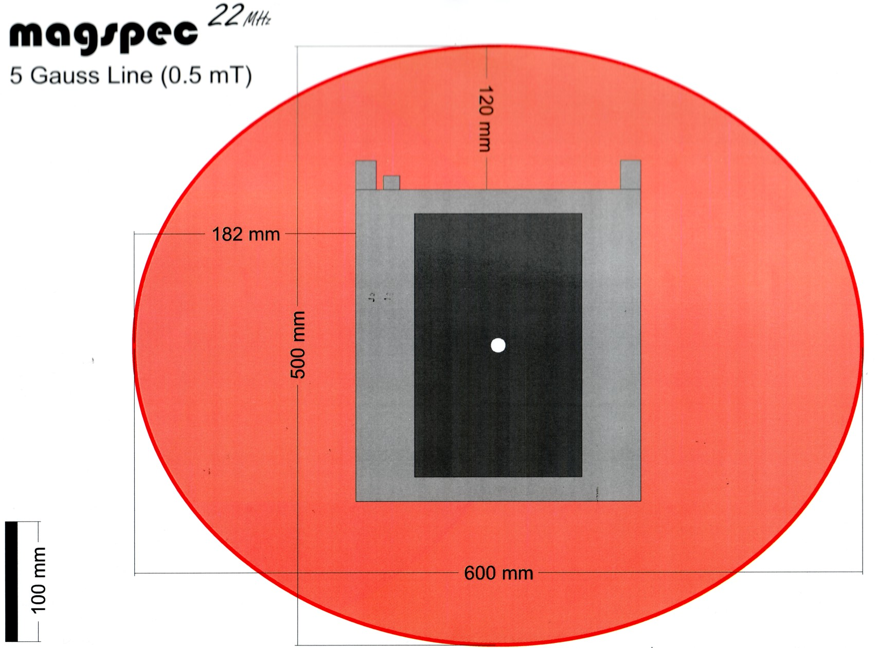
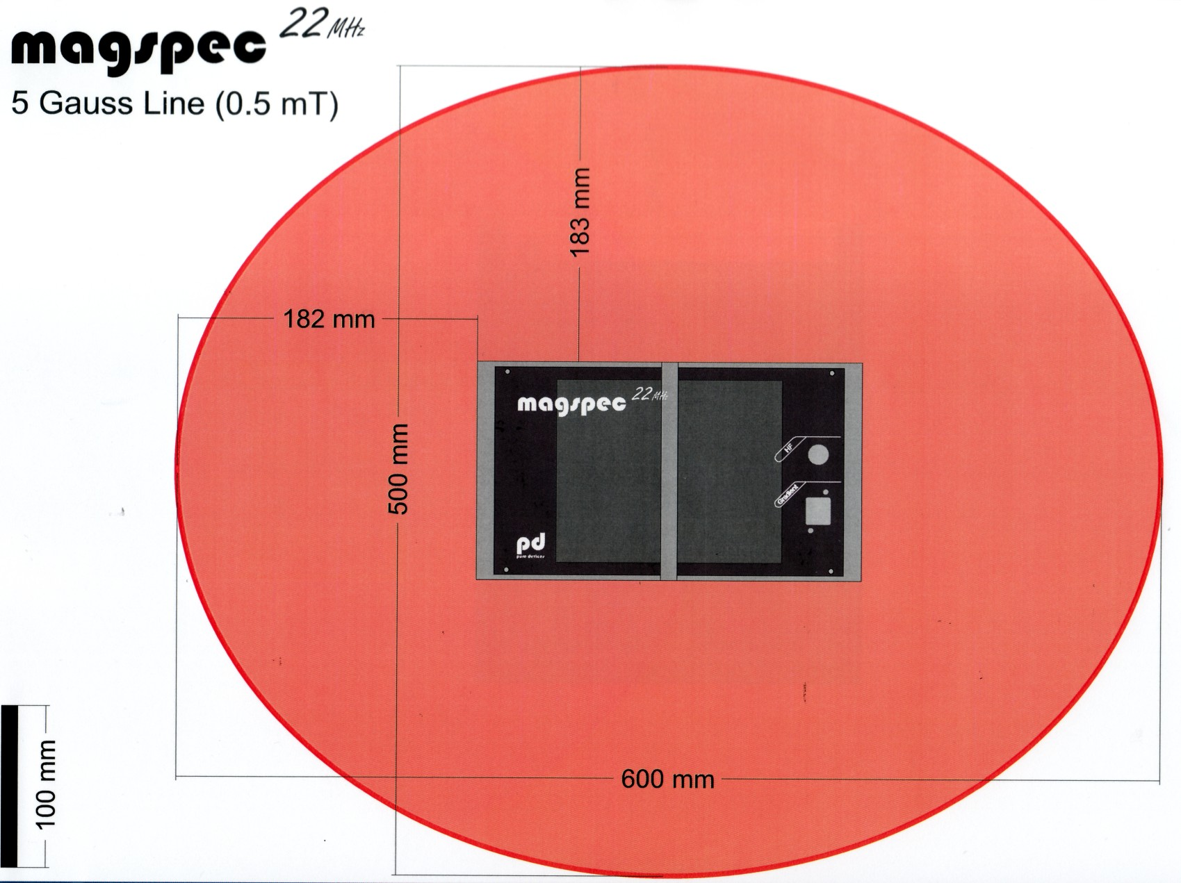
The permanent magnet of the NMR spectrometer is a possible threat for people using a pacemaker or defibrillator and for pregnant women. Under no circumstances should they approach the magnet closer than the 5 Gauss line.